Pitfalls To Avoid When Incorporating Macroeconomic Variables into Forecasts (Part I)
by Michael Surace and Robert Chang
 Forecasting is an integral part of an informed decision-making process for organizations. While any type of future uncertainty can be a subject of forecasting, financial institutions especially strive to predict the impact of future economic conditions. Regulatory stress-testing and accounting frameworks, such as DFAST, CCAR, and CECL, are based on understanding outcomes under different economic scenarios. It is common for financial institutions to build models that forecast default rates, prepayment rates, loss given default, and loan balances based on macroeconomic conditions.
Despite the prevalence of macroeconomic-based forecasting tools, correlating outcomes with macroeconomic time series is a statistically complex process rife with challenges. Organizations must be prepared to understand stationarity, time trends, unit roots, structural breaks, cointegration, and vector error correction models. Naïve linear regression with a macroeconomic time series often leads to spurious regressions and nonsense results[1]. Building forecasting models based on macroeconomic conditions is also computationally challenging. A modeler must evaluate thousands of different macroeconomic time series for inclusion into a model, prepare and transform each time series, and then test different variable combinations as candidate models, which could number into the hundreds of thousands.
Macroeconomic Data and Stationarity
Macroeconomic data generally comes in the form of time series, which makes forecasting inherently challenging due to the statistical complexity called stationarity. In essence, the statistical properties of a stationary time series are constant over time. This is an important feature for forecasting, as traditional statistical models such as regressions generally fail to provide a useful statistical inference under non-stationarity. While the estimation of a statistic (e.g., mean, variance) that is not constant over time has its challenges, non-stationarity also causes other estimation problems. In the following section, we discuss two important problems associated with non-stationary time series: spurious regressions and structural breaks.
Spurious Regressions and Non-Stationarity due to Time Trends
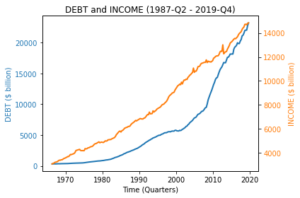
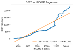
Spurious correlation (or regression) occurs when there is a statistical relation between two variables, but the variables are not causally related. For instance, as the economy grows, both total public debt (DEBT) and real disposable personal income (INCOME) trend upward over time (i.e., the mean value of the time series is not constant, hence non-stationary). The quarterly time series of these two variables for the U.S. economy from 1987-Q2 to 2019-Q4 are plotted in Figure 1[2]. When we model the linear relation between DEBT and INCOME via simple linear regression, we get a very high R-squared value (0.890) and a high statistical significance for the coefficient estimate on INCOME (t-stat = 41.569 and p-value < 0.000). Figure 2 presents the scatter plot and linear regression line for DEBT and INCOME.
| Figure 1 – Time Series of DEBT and INCOME
|
Figure 2 – Regression of DEBT and INCOME
|
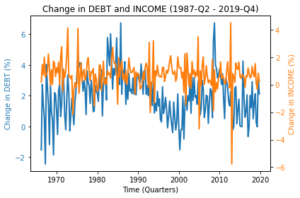
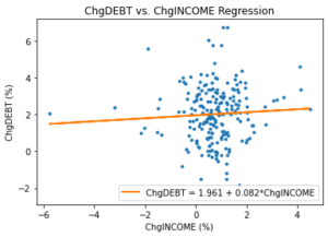
The high statistical correlation does not imply a strong causal link between DEBT and INCOME. To see this, we plot the quarter over quarter percentage change for both time series (ChgDEBT and ChgINCOME), and do not observe any upward trend. The time series are plotted in Figure 3. If we run a linear regression on the changes, the R-squared is very low (0.003). Additionally, the coefficient estimate on INCOME is far from being statistically significant (t-stat = 0.853 and p-value < 0.395). Figure 4 presents the scatter plot and linear regression line for DEBT and INCOME.
| Figure 3 – Time Series of ChgDEBT and ChgINCOME
|
Figure 4 – Regression for ChgDEBT and ChgINCOME
|
More strikingly, a multi-variable regression of DEBT on INCOME and Gross domestic product (GDP) reveals that INCOME and DEBT are negatively related when GDP (a proxy for the size of the economy) is controlled (see Column 1 of Table 1). However, a similar regression setup with change variables does not yield any statistically significant relation. The differences in R-squared values support the notion that the relation among these variables can be mostly attributed to their common trend[3].
Table 1 – Multivariate Regression Results for Level and Change
| |
(1) |
|
(2) |
| |
DEBT |
|
ChgDEBT |
| INCOME |
-4.551 |
ChgINCOME |
0.086 |
|
(0.000) |
|
(0.378) |
| GDP |
3.562 |
ChgGDP |
-0.030 |
|
(0.000) |
|
(0.787) |
| R-squared |
0.969 |
|
0.004 |
| p-values are in parenthesis. |
Overall, non-stationarity due to trending time series may cause serious problems in statistical inference.
Non-Stationarity due to Structural Breaks
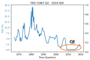
Structural breaks are another source of non-stationarity for macroeconomic time series. In simple terms, structural breaks refer to unexpected abrupt changes in statistical parameters of time series variables. For instance, the quantitative easing period (QE) following the global financial crisis represents a structural break for the effective federal funds rate (FED), depicted in Figure 5. As evident from the figure, the financial crisis caused a structural break in the interest rate environment; interest rates were close to zero with very low variation in the post-financial crisis period. Consequently, statistical modeling efforts using pre-financial crisis period data can lead to large forecasting errors for the post-financial crisis period.
Figure 5 – Time Series of FED
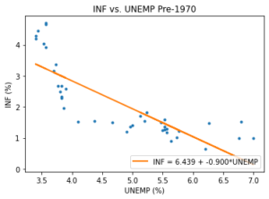
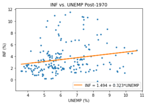
A structural break can also refer to a change in the statistical relationship between two time series. For instance, it is believed that there was a strong inverse relationship between unemployment (UNEMP) and inflation (INF) in the pre-1970 period, and that this relationship has weakened in recent decades[4]. Therefore, the relationship between both time series is not stable, which can cause large forecast errors depending on the period of estimation and forecasting. The scatter plots and accompanying linear regression lines are presented for the pre- and post-1970 periods in Figure 6 and 7, respectively.
| Figure 6 – Regression for INF and UNEMP (Pre-1970)
|
Figure 7 – Regression for INF and UNEMP (Post-1970)
|
While the scatter plot in Figure 6 for the pre-1970 period shows a strong inverse relationship (with curvature), we do not observe such a relationship for the post-1970 period in Figure 7[5]. As such, the relationship between INF and UNEMP appears to have changed significantly, suggesting a potential structural break around 1970.
Testing and Correcting for Non-Stationarity
Stationarity Tests
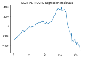
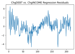
As discussed in the previous section, non-stationary time series can cause problems in statistical inference and forecasting. Although graphical examination is a valuable tool to reveal trends and structural breaks in time series, there are other quantitative tools to test the stationarity of a time series. One commonly used tool is the unit root test. We will not go into the details and underlying theory of unit root testing. However, to give some context, the general idea of unit root testing is to assume a stochastic process for the data and apply hypothesis testing to the parameters of the process to test for stationarity or non-stationarity. Some of the commonly used unit root tests are Augmented Dickey-Fuller (ADF), Kwiatkowski-Phillips-Schmidt-Shin (KPSS), and Phillips-Peron (PP) tests[6]. Unit root tests are generally applied to raw data to check whether they are suitable for regression purposes. Additionally, it is possible to apply unit root tests to the residuals of a regression output as a post-estimation diagnostic for stationarity. If the residuals are non-stationary, one of the assumptions for linear regression is violated and the regression can be spurious. Figures 8 and 9 present the residual plots of the regressions shown in Figure 2 and 4, respectively.
| Figure 8 – Residuals from Level Regression
|
Figure 9 – Residuals from Change Regression
|
It is clear from Figure 8 that the residuals are non-stationary for a naïve regression of DEBT and INCOME levels. However, the residuals in Figure 9, which regress changes of DEBT and INCOME (ChgDEBT and ChgINCOME), behave closer to a stationary process.
Making a Time Series Stationary
While statistical inference is problematic with non-stationary time series, there are certain methods to make a time series stationary. A commonly used method is differencing, which is creating another time series by computing the difference between consecutive observations. In other words, the first difference of a time series is a time series of the changes between consecutive observations.
where yt and Δyt denote the original and first-differenced time series, respectively[7]. This method helps remove certain types of trends from the time series. A similar transformation serves the same purpose: calculating the growth rate between consecutive observations.
|
gyt = (yt – yt–1)/(yt–1) |
(2) |
where yt and gyt denote the original and growth time series, respectively[8]. There are other transformations that can help make a time series stationary, some of which include seasonal differencing, logarithmic transformation, and power transformation. It is also possible to fit a trend model to the time series and use the residuals as the stationary time series.
Is Stationarity Always Necessary? Cointegration and Error Correction Models
When conducting a linear regression analysis, there is an exception to the stationarity condition. This exception happens when time series are cointegrated. In the simple case of two variables, x and y are said to be cointegrated if both time series are non-stationary and there is a linear combination of x and y that is stationary[9]. When the variables are cointegrated, their movements are non-stationary but they move together (e.g., x and y both have an upward time trend, but they are still related). Suppose x and y are time series both integrated of order 1 (i.e., x~I(1) and y~I(1)) and also cointegrated. We can write
and
where u is stationary (i.e., u~I(0)) and (1, -α, -β) is called the cointegrating vector. In that case, we can estimate the linear regression coefficients by Ordinary Least Square (OLS), and the coefficient estimates will be consistent (i.e., converge to true value)[10]. However, the coefficient estimates will not follow a normal or student’s t distribution. Consequently, OLS can be used to estimate coefficients but not for statistical testing. To use standard inference techniques, we utilize an error correction model (ECM). An example ECM can be defined as
|
Δyt = κ + y1Δyt–1 + β0Δxt + β1Δxt-1 + δût–1 + εt |
(5) |
Since all the terms are stationary in Equation 5, we can use the standard OLS techniques for both estimation and testing [11]. The general idea of the model is that the short-term deviation (which is represented by ut) from the long-term equilibrium (represented by Equation 3) is corrected at a speed determined by the coefficient estimate on ut.
In Part II of this discussion to be released on September 13th, we introduce an automated tool that we built for regressing any variable of interest (e.g., default rate, prepayment rate) against macroeconomic factors. The tool is based on FI’s deep experience in building macroeconomic-based forecasting models in various public and private sector settings. The tool eliminates time-consuming manual steps in the variable selection process and ensures that forecast models based on macroeconomic variables are statistically valid.
References:
[1] Granger, C.W.J. and Newbold, P. (1974) Spurious Regressions in Econometrics. Journal of Econometrics, 2, 111-120
[2] We truncated our sample period in 2019 to exclude certain extreme values related to COVID-19 macroeconomic policies.
[3] The regressions in Table 1 can still be mis-specified due to other violations of linear regression assumptions (e.g., omitted variables).
[4] The inverse relation between inflation and unemployment is also known as Phillips Curve, which has “flattened” in recent decades.
[5] Indeed, the positive coefficient estimate on UNEMP is statistically significant.
[6] This is not an exhaustive list of stationarity tests. There are other unit root tests and/or their variations (e.g., ADF test with drift and deterministic trend). Additionally, there are other visual tools (e.g., auto-correlation functions) and non-parametric tests for checking stationarity of a time series.
[7] It is also possible to difference a series more than once. For instance, second difference of yt would correspond to first difference of Δyt.
[8] While growth time series is easier to interpret than first difference time series, growth rates may not be meaningful for interval scale variables (e.g., credit scores).
[9] In the case of two variables, cointegration requires both variables to have the same order of integration, which is defined as the minimum number of differencing operation required to make a time series stationary. For instance, if x is integrated of order 2 (i.e., x ~ I(2)), then the series should be differenced twice to make it stationary. In the case of more than two variables, the order of integration does not need to be the same for all variables. However, certain conditions should still hold such that there exists a linear combination of the variables that is stationary.
[10] Indeed, the coefficient estimate will be super consistent and converge to the true value at a faster rate than the standard OLS estimator.
[11] The model can be generalized such that the right-hand side can include up to p and q lags of x and y variables, respectively. We will not go into the details of how to choose the number of lags optimally. It is also possible to extend the model to a multivariate version, which is called vector error correction model (VECM).