Pitfalls to Avoid When Incorporating Macroeconomic Variables Into Forecasts (Part II)
By Michael Surace and Robert Chang
 Despite the prevalence of macroeconomic-based forecasting tools, correlating outcomes with macroeconomic time series is a statistically complex process rife with challenges (see Part I). Organizations must be prepared to understand stationarity, time trends, unit roots, structural breaks, cointegration, and vector error correction models. Naïve linear regression with a macroeconomic time series often leads to spurious regressions and nonsense results[1]. Building forecasting models based on macroeconomic conditions is also computationally challenging. A modeler must evaluate thousands of different macroeconomic time series for inclusion into a model, prepare and transform each time series, and then test different variable combinations as candidate models, which could number into the hundreds of thousands.
FI Consulting built an automated tool for regressing any variable of interest (e.g., default rate, prepayment rate) against macroeconomic factors, based on our deep experience in building macroeconomic-based forecasting models in various public and private sector settings. Our tool searches through a long list of candidate macroeconomic variables based on business line preferences and automatically prepares the variables for regression, checking stationarity, cointegration, and structural breaks. The tool then tests candidate models and ranks them based on goodness-of-fit. The business line can then select the model best suited for the business purpose, remain confident that the model is statistically sound, and that the model passes statistical tests.
In the following sections, we demonstrate how our tool overcomes the statistical challenges of building macroeconomic-based forecasting models. We walk through examples of using our tool to forecast mortgage portfolio delinquency rates and consumer loan charge-off rates under different economic environments. While we use mortgage delinquency rates and consumer loan charge-off rates as examples, we designed our tool to forecast any dependent variable of choice based on any number of potential macroeconomic variables as predictors.
1 FI’s Solution
As described in Part I, incorporating macroeconomic variables into a business’s forecasting processes is statistically challenging and requires significant resources to implement correctly. To reduce the level of effort institutions face, FI has developed a tool that automates the building of macroeconomic-based forecasting models. FI designed the tool to accept any dependent variable of interest, prepare macroeconomic variables for regression analysis, and output a set of candidate models that are accurate and statistically sound. The remainder of this section discusses the capabilities of FI’s automated tool, the value it provides to financial institutions, and analyzes the tool’s performance when used to forecast two different variables, a mortgage portfolio delinquency rate and consumer loan charge-off rate. The diagram below provides an overview of the automated model-building process.
To show an instance of macroeconomic-based forecasting with non-stationary time series, we apply the tool for forecasting a mortgage portfolio delinquency rate and consumer loan charge-off rate regressed on several macroeconomic factors. While we use mortgage delinquency rates and consumer loan charge-offs in this example, we designed the tool to forecast any dependent variable of choice based on any number of potential macroeconomic variables as predictors. This section first discusses how to prepare and transform the data to ensure that the model is statistically sound. Next, we discuss selecting our predictor variables and evaluating candidate models. Finally, we apply our model to forecasting a mortgage portfolio delinquency rate and consumer charge-off rate and discuss the results.
Data Preparation
We designed the tool to predict any dependent variable of choice and develop forecast models using relevant macroeconomic variables as independent variables. The tool houses a suite of raw, publicly available historical macroeconomic data for building forecast models[2]. The data covers a broad spectrum of macroeconomic variables, including interest rates, housing market variables, consumer debt, consumer sentiment, and monetary data.
We first import macroeconomic data and put it in a panel format (each column representing a time series of a different variable). Next, we select our dependent variable (y) and independent variables (X). Then, for each independent variable, we create transformations, including lags, differences, and growth rates[3]. The diagram below provides an illustration of the types of transformations that are performed on the macroeconomic data.
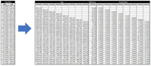
Transformations of each macroeconomic variable significantly expand the number of possible predictors for estimation and can be a resource expensive exercise. A modeler must conduct a series of tests on each variable to determine which transformation will do the best job at predicting the dependent variable. Automating this step is critically important, as a manual approach would severely restrict the number of macroeconomic variables available for consideration.
Unit Root Testing
Once the data is imported and prepared, we must analyze it to determine if it can be used in regression analysis. One of the main issues with time series data is the presence of a unit root. That is, the data series is non-stationary and exhibits changes in the mean, variances, and covariance over time. Non-stationary data used in regression analysis can lead to biased predictions. The tool conducts three different statistical tests to check for stationarity in each time series:
- Augmented Dickey-Fuller (ADF) Test: Null Hypothesis that a unit root is present in the time series. Failure to reject the null hypothesis concludes that the time series is non-stationary.
- Kwiatkowski-Phillips-Schmidt-Shin (KPSS) Test: Null hypothesis that a unit root is not present in the time series. Failure to reject the null hypothesis concludes that the time series is stationary.
- Phillips-Perron (PP) Test: Null Hypothesis that a unit root is present in the time series. Failure to reject the null hypothesis concludes that the time series is non-stationary.
For each macroeconomic variable, we follow the process below:
- Run all three unit roots tests to check for stationary. There are instances where each test’s conclusion may differ; when this happens, the model uses a “Majority Vote” rule. That is, if two or more of the unit root tests conclude the data series is stationary, then the model will classify the variable as stationary. Otherwise, the variable will be classified as non-stationary.
- Discard all variables that are classified as non-stationary.
The result of this process is a pool of macroeconomic variables and transformations that are stationary. These variables will be used as predictors in the forecast models.
Variable Selection
Once the model has identified the pool of candidate variables that can be used in the regression models, we must identify which combination of variables produces the “best” models. The tool uses the Best Subsets algorithm to identify candidate variables[4]. The algorithm tests every possible combination of variables and, based on a defined criterion, selects the variable groupings that perform the best. For example, if we have 3 variables, we will fit separate models for all possible combinations of three variables. This approach is advantageous because it tests all possible variable groupings. Once all possible combinations of “n” predictors have been specified, the model reduces the number of candidate models using the following approach:
- Removes models that do not consider a diverse set of macroeconomic data. For example, a model that used three different transformations of GDP would be removed. This is to ensure that the final model considers different types of macroeconomic indicators.
- Removes models where the residuals are non-stationary. This ensures that we do not violate the assumptions of linear regression, utilizes OLS for estimation.
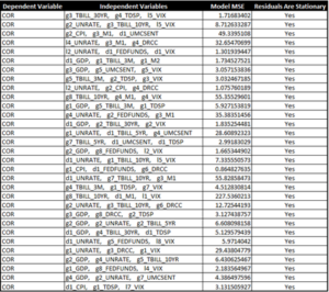
After the model has removed candidate models that contain redundant predictors and ones that do not have stationary residuals, the tool selects the best candidate based on a specified testing criterion, such as the candidate models with the highest adjusted R2 or lowest residual sum of squares (RSS). This approach is advantageous because every possible combination of variables gets tested; however, when working with a large number of predictors, the number of possible combinations can be immense. In general, if there are k predictors, there are 2k possible combinations. This approach can be very resource and time intensive. The diagram below illustrates the resulting dataset that is created after the best subset algorithm is executed and the filtering process has been completed.
Forecasting Model
Once we identify the optimal predictors of the dependent variable, the tool runs a final regression on the dependent variable. In this model, we use the predictor variables observed at time t (Xt,1, Xt,2, … Xt,K) to forecast Yt in a classical linear regression setting[5]. The model can be summarized in Equation as follows:
|
Yt = β0 + β1Xt,1 + β2Xt,2 + ⋯ + βKXt,K + ϵt |
|
We estimate the coefficients (β’s) by OLS. The model’s estimation window is fixed. For instance, suppose we have 100 observations in our time series data; we use the first 70 observations to estimate the coefficients. Following the estimation procedure, we use the same estimated coefficients to predict the values of the dependent variable for the remaining observations. This is equivalent to splitting our data into training and testing datasets[6].
2 Forecasting Results
In order to assess the performance of The Model we ran the algorithm on two sets of dependent variables; 1) Mortgage Delinquency Rates, and 2) Consumer Loan Charge Off Rates. The model results are presented in the following sections.
Mortgage Delinquency Rates
We pulled quarterly mortgage delinquency rates (MDR) from FRED for the period 1991 to 2021. The tool trained the regression on data from 1991 to 2013. We selected the final specification presented below:
|
MDRt = β0 + β1DiffCPIt + β2GrowthUMCSENTt-5 + β3GrowthVIXt-4 + ∈t |
|
where,
DiffCPI = First difference of CPI
GrowthUMCSENT = 5 Quarter lag of US consumer sentiment
GrowthVIX = 4 quarter growth rate of the VIX index
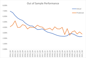
The figure below shows the model prediction compared to the actual rates for the hold-out period.
Figure 1. Mortgage Delinquency Rates Out of Sample Performance
Consumer Loans Charge-off Rate
We pulled quarterly consumer loan charge-off rates (COR) from FRED for the period 1987 to 2021. The model trained the regression on data from 1987 to 2013. We selected the final specification presented below:
|
CORt = β0 + β1GrowthFEDFUNDSt–8 + β2GrowthDRCCt–8 + β3VIXt–8 + ∈t |
|
where,
GrowthFEDFUNDS = 8 quarter growth rate of the Federal Funds rate
GrowthDRCC = 8 Quarter growth rate of the delinquency rate of credit cards
VIX = 8 quarter lag of the VIX index
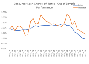
The figure below shows the model prediction compared to the actual rates for the hold-out period.
Figure 2. Consumer Loan Charge-off Rates Out of Sample Performance
Conclusion
Incorporating macroeconomic variables into a business’s forecasting processes is statistically challenging and requires significant resources to implement correctly [Macroeconomics – Part I]. To reduce the level of effort institutions face, FI has developed a tool that automates the building of macroeconomic-based forecasting models. Interested in learning more or reviewing if your institutions models are implemented correctly? Email Robert Chang and Michael Surace at [email protected].
References:
[1] Granger, C.W.J. and Newbold, P. (1974) Spurious Regressions in Econometrics. Journal of Econometrics, 2, 111-120
[2] The historical macroeconomic data is pulled from FRED (https://fred.stlouisfed.org/).
[3] While it is possible to create infinitely many transformations, we created lags up to 8 periods, and first difference and growth rates up to 8 periods.
[4] Furnival, G. M., and Wilson, R. W. (1974). “Regression by Leaps and Bounds.” Technometrics 16:499–511.
[5] The model allows for contemporaneous relationships between the dependent and independent variables. Under this design, we assume that macroeconomic forecasts are perfect. This is a common assumption used by institutions when forecasting.
[6] Note, The Model currently uses 70% of the observations to train the regression and the remaining 30% as the hold-out sample. However, this can be configured by the user.